Sample Partition

The balanced_partition() function partitions samples into balanced groups while minimizing variance in group means and standard deviations. This is useful for creating balanced experimental groups, cross-validation folds, or training/test splits.

Overview

The partitioning algorithm minimizes:

$\text{loss} = \text{Gini}(\text{group\_means}) + \lambda \times \text{Gini}(\text{group\_SDs})$

where:

Gini(group_means) measures inequality in group means
Gini(group_SDs) measures inequality in group standard deviations
lambda controls the trade-off between balancing means vs. SDs

Basic Usage

Simple partition

library(Rtoolset)

# Load external data
data_file <- system.file("extdata", "8988T.csv", package = "Rtoolset")
data <- read.csv(data_file)

head(data)
#>   NO.    L   W   BW
#> 1 221  8.8 7.7 19.8
#> 2 222 10.4 8.1 21.8
#> 3 223  9.2 8.4 20.6
#> 4 224  8.2 7.2 21.8
#> 5 225  9.2 8.1 20.4
#> 6 226  8.3 6.8 24.9

# Partition into 4 balanced groups based on BW (body weight)
result <- balanced_partition(
  data = data,
  score_col = "BW",
  id_col = "NO.",
  K = 4
)

# View the assignment
head(result$assignment)
#>    sample_id group score
#> 3        223     1  20.6
#> 9        231     1  22.5
#> 13       236     1  25.8
#> 15       238     1  24.7
#> 17       241     1  23.7
#> 18       242     1  25.3

With Custom Group Sizes

# Specify exact group sizes
result <- balanced_partition(
  data = data,
  score_col = "BW",
  id_col = "NO.",
  group_sizes = c(6, 6, 6, 6)  # Must sum to the total number of samples
)

Advanced Options

Adjusting the Balance Trade-off

The lambda parameter controls how much weight to put on balancing standard deviations:

# Emphasize mean balance (default lambda = 1)
result1 <- balanced_partition(
  data = data,
  score_col = "BW",
  K = 4,
  lambda = 0.5  # Less weight on SD balance
)

# Emphasize SD balance
result2 <- balanced_partition(
  data = data,
  score_col = "BW",
  K = 4,
  lambda = 2.0  # More weight on SD balance
)

Partition Methods

Two methods are available:

# Blocked permutation (default, faster for large datasets)
result1 <- balanced_partition(
  data = data,
  score_col = "BW",
  K = 4,
  method = "blocked_permute"
)

# Random assignment (more thorough search)
result2 <- balanced_partition(
  data = data,
  score_col = "BW",
  K = 4,
  method = "random_assign",
  B = 10000  # More iterations for better results
)

Output Options

Save plots and CSV files to a directory:

result <- balanced_partition(
  data = data,
  score_col = "BW",
  id_col = "NO.",
  K = 4,
  output_plot = TRUE,       # Generate visualization
  output_csv = FALSE,       # Set to TRUE to save CSV file
  output_dir = NULL,        # Set to directory path to save files
  file_prefix = "partition" # File prefix
)

Understanding the Results

The function returns a list with several components:

result <- balanced_partition(data, score_col = "BW", K = 4, output_plot = TRUE)

# Assignment: which group each sample belongs to
result$assignment
#>    sample_id group score
#> 1          1     1  19.8
#> 6          6     1  24.9
#> 10        10     1  24.3
#> 12        12     1  25.6
#> 21        21     1  22.6
#> 23        23     1  23.5
#> 3          3     2  20.6
#> 7          7     2  25.3
#> 13        13     2  25.8
#> 16        16     2  24.7
#> 19        19     2  23.9
#> 20        20     2  22.5
#> 2          2     3  21.8
#> 4          4     3  21.8
#> 11        11     3  23.3
#> 15        15     3  24.7
#> 18        18     3  25.3
#> 22        22     3  26.2
#> 5          5     4  20.4
#> 8          8     4  24.7
#> 9          9     4  22.5
#> 14        14     4  25.7
#> 17        17     4  23.7
#> 24        24     4  24.9

# Group statistics: mean, SD, and n for each group
result$group_stats
#>   group   score.n score.mean  score.sd
#> 1     1  6.000000  23.450000  2.073403
#> 2     2  6.000000  23.800000  1.949359
#> 3     3  6.000000  23.850000  1.846889
#> 4     4  6.000000  23.650000  1.936750

# Loss value: lower is better
result$loss
#> [1] 0.03430415

# Group sizes used
result$group_sizes
#> [1] 6 6 6 6

# Plot object (if output_plot = TRUE)
result$plot
#> Bin width defaults to 1/30 of the range of the data. Pick better value with
#> `binwidth`.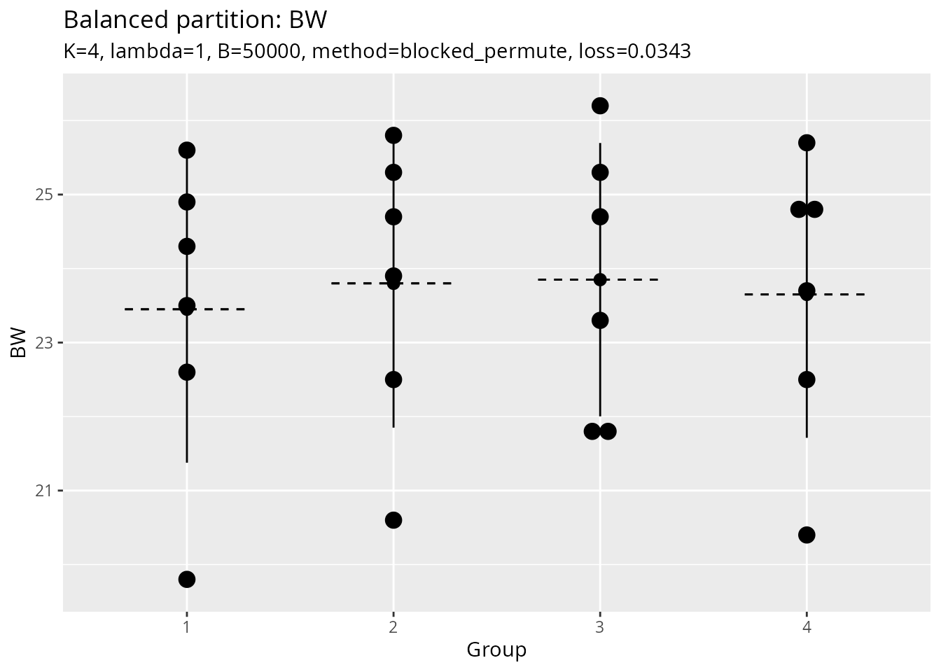

Use Cases

1. Experimental Design

Create balanced treatment groups:

# Create 4 balanced treatment groups using body weight
groups <- balanced_partition(
  data = data,
  score_col = "BW",
  id_col = "NO.",
  K = 4,
  output_plot = TRUE
)

2. Data Splitting for Train/Test

Create balanced splits for cross-validation or train/test sets:

# Cross-validation: Create 5-fold CV with balanced groups
cv_folds <- balanced_partition(
  data = data,
  score_col = "BW",
  K = 5
)

# Use the groups for cross-validation
for (fold in 1:5) {
  test_indices <- which(cv_folds$assignment$group == fold)
  train_indices <- which(cv_folds$assignment$group != fold)
  # ... perform CV ...
}

# Training/Test Split: 80/20 split (approximately 19 and 5 samples)
split <- balanced_partition(
  data = data,
  score_col = "BW",
  group_sizes = c(19, 5)
)

train_data <- data[split$assignment$group == 1, ]
test_data <- data[split$assignment$group == 2, ]

Tips and Best Practices

Data Quality: Ensure your score column has no missing values
Group Sizes: For best results, groups should be roughly equal in size
Lambda Tuning: Start with lambda = 1, adjust based on your needs
Reproducibility: Use seed parameter for reproducible results
Visualization: Always check output_plot = TRUE to verify balance

Algorithm Details

The core algorithm (balance_partition_core) uses a random search approach:

Generate candidate partitions using the selected method
Evaluate each partition using the Gini-based loss function
Iterate through candidates and return the partition with the lowest loss

The number of candidates (B) can be increased for better results at the cost of computation time.